Bayesian Analysis of Syntopy

Assignment for Bayesian Statistics Course

Syntopy

Simulated Data

Bayesian Inference

Author

Matěj Tvarůžka

Published

June 27, 2026

1 Introduction

Following the framework of Remeš and Harmáčková (2023), this assignment simulates and analyses local co-occurrence (syntopy) among sister species of birds. In evolutionary ecology, syntopy is the final stage of the speciation cycle, during which two sister species meet at the same sites within their range overlap. This process leads to build-up of local biodiversity over time and is driven by niche conservatism, ecological specialisation and energetic constrains (Remeš and Harmáčková 2025).

In this work, I model the co-occurrence affinity at local sites as a function of ecological and spatial predictors. This idea is connected to the topic of my master’s thesis, in which I model syntopy at two spatial scales using BBS (Breeding Bird Survey) data for passerines and eBird Status & Trends range maps. Therefore, I decided to simulate data to match the design of the BBS data to understand their structure and modelling options better.

Assignment Goals

Generate dream syntopy data for both scales (routes and stops).
Visualise and explore generated data.
Fit models for both scales using the ulam() function and compare the estimates with true values.

To measure syntopy accurately, we need to consider only sites within the range overlap for the analysis, because otherwise it will lead to biased results (Remeš and Harmáčková 2023). We can imagine the range overlap being the jar, from which we randomly draw balls (sites with a particular co-occurrence state of both species). There are four possible outcomes of that draw:

Both species are present,
Species A is present,
Species B is present,
Both species are missing at the site.

If we want to model this problem using Bayesian methods, than the most accurate probability distribution for our problem is Fisher’s non-central hypergeometric distribution, because the sampling is carried out without replacement, which reflects the true nature of the problem, given the limited number of pairs. We can follow the Bayesian approach in Newbury (2025) measuring the degree of species co-occurrence with the log-odds ratio (for details see box 1).

Box 1: Bayesian Log Odds Ratio

The log-odds ratio serves as the foundational metric to quantify spatial association between sister species. Based on a standard \(2 \times 2\) presence-absence matrix (\(a\) = both present, \(b/c\) = single species present, \(d\) = both absent), the empirical calculation is:

\[\log \text{OR}_{\text{}} = \ln\left(\frac{a \times d}{b \times c}\right)\]

In this assignment, we transition away from this traditional empirical formula and instead implement a Bayesian framework. The key distinctions and advantages are:

Mathematical Formulation:

The observed co-occurrence \(k_i\) is modelled with Fisher’s Hypergeometric distribution representing local survey plots within that site: \[k_i \sim \text{FisherHypergeometric}(m_{1i}, m_{2i}, N_i, \alpha_i)\]

where:
- \(k_i\) = number of sites where both species co-occur
- \(m_{1i}\) = total number of sites where species A is present for pair \(i\)
- \(m_{2i}\) = total number of sites where species B is present for pair \(i\)
- \(N_i\) = total number of sites sampled within the sympatric range of pair \(i\)
- \(\alpha_i\) = the conditional co-occurrence odds ratio for pair \(i\).
For each site \(i\) out of \(N\), the co-occurrence affinity (\(\alpha_i\)) is the log-odds ratio of given parameters:

\[\text{log}(\alpha_i) = \beta_{0} + \beta_{1} \cdot X_{1,i}\]
Mathematical Stability: By evaluating data through the Log Probability Mass Function (LPMF) of Fisher’s Non-Central Hypergeometric distribution, our model naturally handles small sample sizes and zero counts. It completely bypasses the need to delete data or inject mathematical bandages.
Symmetric Linear Predictors: Taking the natural logarithm maps highly asymmetric raw odds ratios onto a continuous linear space from \(-\infty\) to \(+\infty\), centering independent sorting perfectly at \(0\) (\(>0\) is syntopy, \(<0\) is allotopy). This allows our ecological parameters (\(\beta_{\text{res}}\), \(\beta_{\text{hab}}\), etc.) to be added together seamlessly.
Prevalence Invariance: Unlike traditional similarity indices (e.g., Jaccard, Simpson), this metric standardises for baseline regional abundance, therefore isolates true ecological affinity without being biased by widespread or ubiquitous species.

2 Data Simulation

To satisfy the assignment’s complexity requirements, I define 5 true parameters that dictate the data-generating process:

\(\beta_{0} = 0.5\) (Baseline log-odds of co-occurrence; slight facilitation)
\(\beta_{res.div} = 0.7\) (Resource use divergence: greater divergence increases syntopy)
\(\beta_{hab.pref} = -0.6\) (Difference in micro-habitat and environmental preference decreases syntopy)
\(\beta_{prod} = 0.3\) (Environmental productivity (e.g., NDVI): richer environments facilitate synotopy)
\(\beta_{sympatry} = 0.8\) (Spatial overlap: regional overlap strongly increases syntopy)

I want to simulate data that resembles the BBS study design (for details see box 2). Therefore, I need to create two data sets:

1) route scale (looking at syntopy across transects within the range overlap)

2) stop scale (looking at syntopy within transects).

Box 2: BBS Design and Syntopy Scales

The BBS is a long-term, large-scale, international avian monitoring program initiated in 1966 to track the status and trends of North American bird populations. Volunteers count birds on ~40 km long routes, each with 50 stops. The stops are about 800 meters apart, and birds are counted for 3 minutes within a 400-meter radius at each stop. This approach allows us to compare syntopy at both the stop-scale and the route-scale, which is illustrated below.

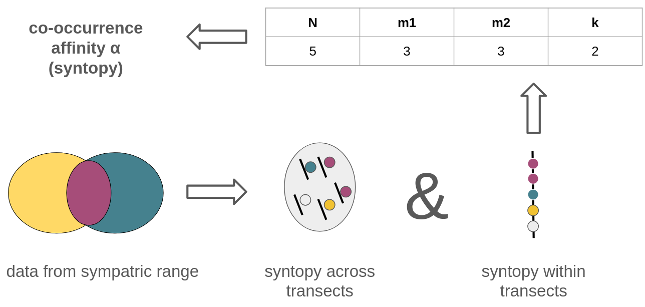
For Fisher’s non-central hypergeometric distribution we can use the library BiasedUrn, and for the modelling, we will use libraries rethinking and rstan. For data wrangling we will use library dplyr. For more advanced visualisations we will use libraries ggplot2 and bayesplot.

library(BiasedUrn)
library(rethinking)
library(rstan)
library(dplyr)
library(ggplot2)
library(bayesplot)
set.seed(1)

2.1 Route Scale

For the routes, I choose a negative binomial distribution because it is integer-valued and has a long right tail. I reflected on the situation in which most species pairs have relatively few routes that could be counted. This is because they mostly do not overlap completely (remember that we take only routes within the range overlap), and also because one or both species should be rather rare rather than common (given the general species-abundance distribution).

For the occupancy-frequency distribution, I decided to use the beta-binomial distribution, which results in an unimodal distribution. However, I acknowledged that the usual shape of the occupancy-frequency distribution is rather biomodal, but the unimodal is also a feasible option (McGeoch and Gaston 2002).

num_pairs <- 100
route_occupancy <- function(num_pairs){
  # simulates the occupancy of species across N routes
  
  # N of routes
  N <-  rnbinom(n = num_pairs, mu = 100, size = 2)
  # Probability distribution for species occupancy
  prob_m1 <- rbeta(num_pairs, shape1 = 1, shape2 = 2)
  prob_m2 <- rbeta(num_pairs, shape1 = 1, shape2 = 2)
  # Species occupancy
  m1 <- rbinom(num_pairs, size = N, prob = prob_m1)
  m2 <- rbinom(num_pairs, size = N, prob = prob_m2)
  list(N=N, m1=m1, m2=m2)
}
route_oc <- route_occupancy(num_pairs = num_pairs)

hist(route_oc$N, breaks = 12, main="N Sites Distribution", xlab="Number of sites for sister pair", col="darkseagreen4")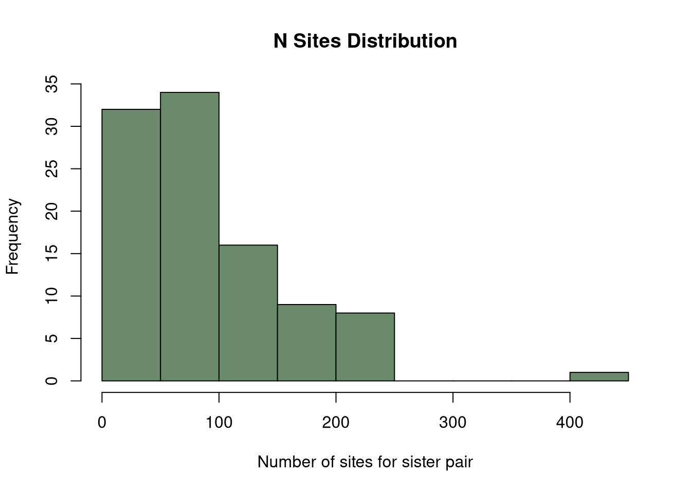

Some species pairs have a very large number of sampled sites, while others have just a few within the sympatric range. We can check the parameters of the distribution:

summary(route_oc$N)

   Min. 1st Qu.  Median    Mean 3rd Qu.    Max. 
   3.00   37.00   73.00   89.89  128.75  407.00

We can also check the occupancy distribution of the first species set in the pairs:

hist(route_oc$m1, breaks = 12, main="Species Occupancy Sample", xlab="Number of occupied routes", col="brown3")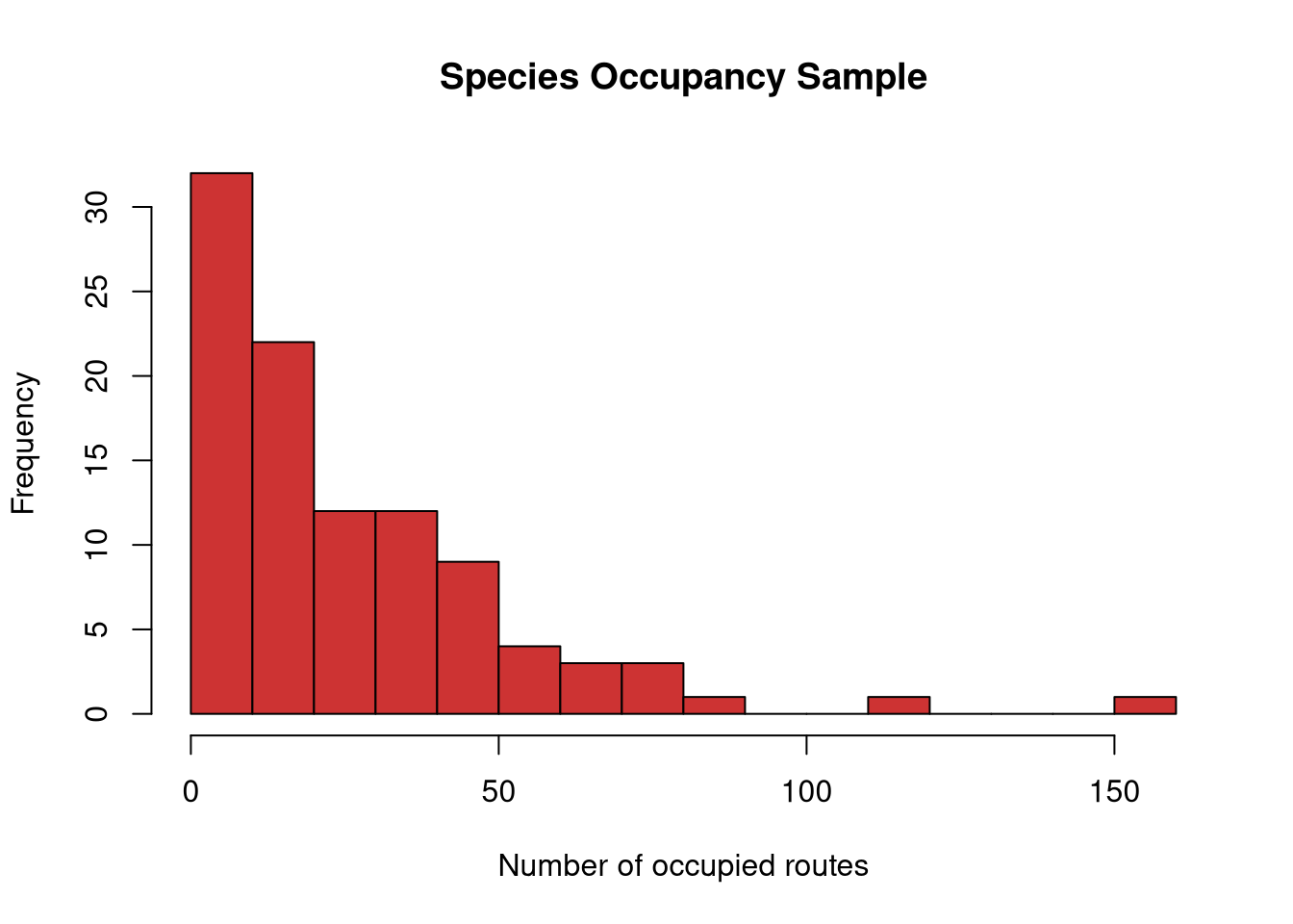

Let us continue with parameter generation. First, I will generate three already standardised variables using a normal distribution.

X_res_div   <- rnorm(num_pairs, mean = 0, sd = 1) # X1
X_hab_pref  <- rnorm(num_pairs, mean = 0, sd = 1) # X2
X_prod      <- rnorm(num_pairs, mean = 0, sd = 1) # X3
hist(X_res_div, breaks = 12, main="Resource Use Divergence", xlab="Degree of divergence", col="orange")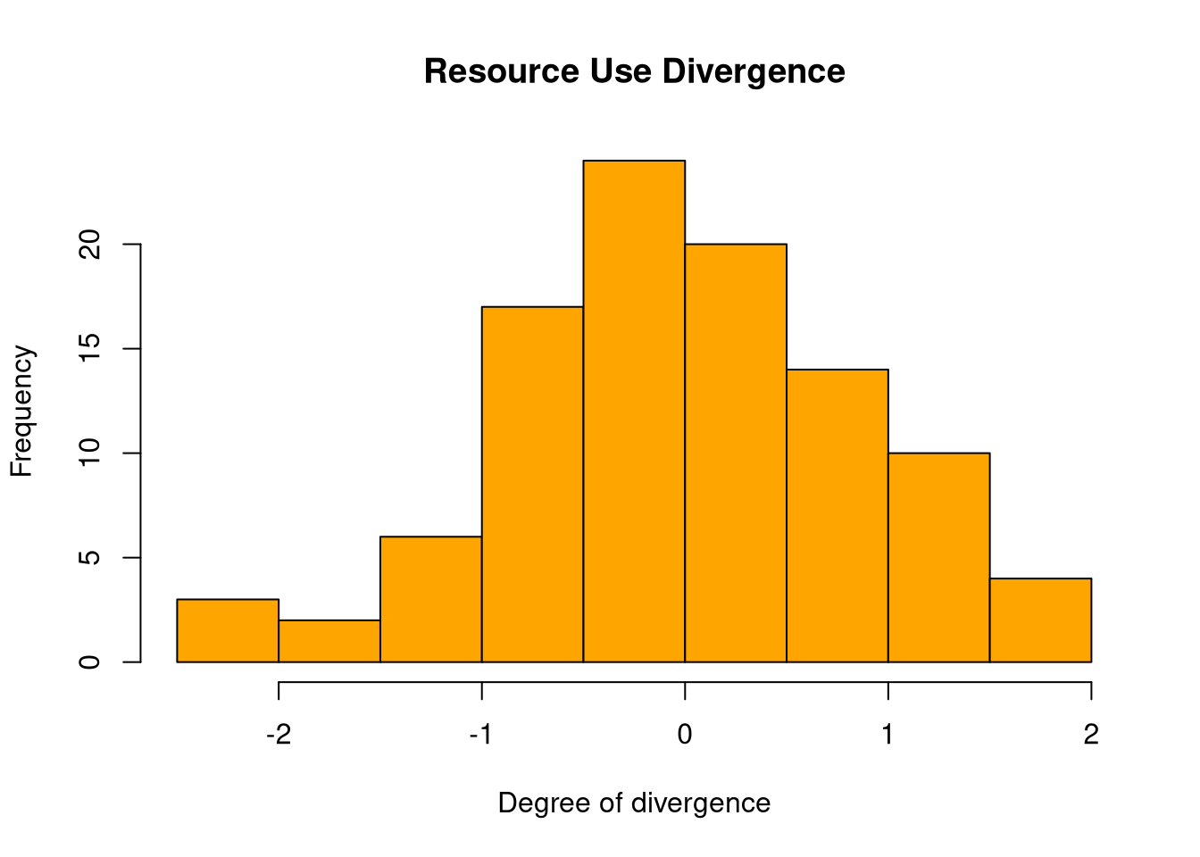

For the degree of sympatry (% of range overlap), I need to generate a distribution with x > 5 (the minimum degree of sympatry is typically 5 %) and x <= 100. As I want the values to have decimals and I need a strict upper limit, I have to use a beta distribution.

raw_beta <- rbeta(num_pairs, shape1 = 2, shape2 =3)
sym_min <- 5 # sympatry threshold is 5 %
symp_max <- 100 # full overlap
sympatry <- sym_min + (raw_beta - min(raw_beta)) * (symp_max - sym_min) / (max(raw_beta) - min(raw_beta))
hist(sympatry, breaks = 12, main="Degree of Sympatry", xlab="Range overlap (%)", col="darkseagreen3")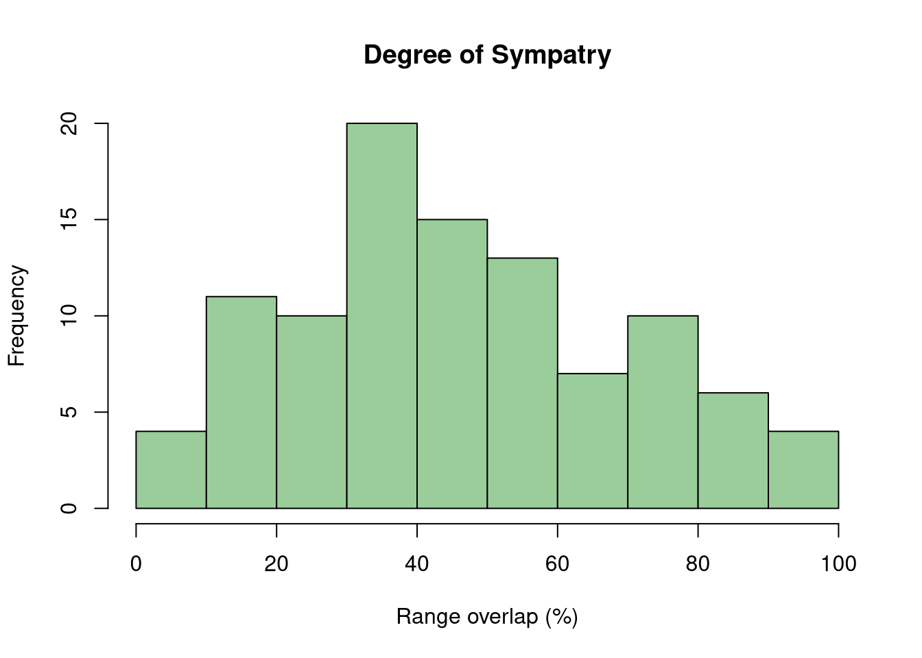

We can see that most pairs have a high degree of sympatry, while a few have very low values. We have to standardise it prior to modelling.

X_sympatry <- (sympatry - mean(sympatry)) / sd(sympatry) # X3
hist(X_sympatry, breaks = 12, main="zSympatry (Standardised)", xlab="Z-score", col="steelblue")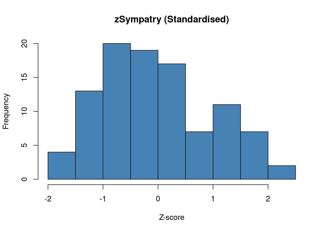

Now we set the “true” parameter values in our made-up universe.

beta_0        <- 0.5
beta_res_div  <- -0.7
beta_hab_pref <- 0.6
beta_sympatry <- 0.8
beta_prod     <- 0.3

The next step is to calculate a linear combination of parameters, and we exponentiate the log-odds ratio to obtain a simple odds ratio.

log_alpha <- beta_0 + 
             beta_res_div  * X_res_div + 
             beta_hab_pref * X_hab_pref + 
             beta_sympatry * X_sympatry + 
             beta_prod     * X_prod
alpha <- exp(log_alpha) # Odds Ratio
summary(alpha)

   Min. 1st Qu.  Median    Mean 3rd Qu.    Max. 
 0.1117  0.6853  1.5003  4.2152  4.2353 41.9001

With this settled, we calculate the linear predictor for each pair using the BiasedUrn library. We will use rFNCHypergeo() function, which uses a slightly different parametrisation of Fisher’s non-central hypergeometric distribution (from the one we will use for modelling), where \(m_1\) is the number of sites with the presence of species A, \(m_2\) is the number of sites with the absence of species B and \(n\) is the total number of sites with the presence of species B.

m1 <- route_oc$m1
m2 <- route_oc$m2
k <- integer(num_pairs)
for(i in 1:num_pairs) {
  set.seed(1)
  # Simple safety boundary: if a species isn't present at all, co-occurrence is 0
  if(m1[i] == 0 || m2[i] == 0) {
    k[i] <- 0
  } else {
    # rFNCHypergeo(n_samples, m1, m2, total_draws, odds)
    k[i] <- rFNCHypergeo(1, route_oc$m1[i], route_oc$N[i] - route_oc$m1[i], route_oc$m2[i], alpha[i])
  }
}

Let us pack it up into data.frame and take a look at the data.

route_data <- data.frame(
  N = route_oc$N, m1 = m1, m2 = m2, k = k,
  res_div = X_res_div, hab_pref = X_hab_pref,
  prod = X_prod, 
  sympatry = X_sympatry
)
head(route_data)

N	m1	m2	k	res_div	hab_pref	prod	sympatry
50	13	22	6	0.5941965	-0.4349607	-0.1926103	0.8118863
178	59	12	4	-0.2703152	-0.5217542	1.6831539	-0.6219037
204	34	39	4	1.5540761	0.9922884	0.1025738	-0.0714691
111	74	8	7	-0.5107425	-1.0854224	-0.6548353	0.4832526
30	9	24	9	-0.2918427	0.9598324	1.1865752	0.2616068
57	14	42	11	1.1014382	-1.0390105	-1.2723697	1.2241687

The route_data looks good, and we can now explore the data before proceeding to the next stage.

nrow(route_data[route_data$k == 0,])

[1] 15

# There is 15 pairs with k=0
route_data[abs(route_data$m1 - route_data$m2) >100,]

	N	m1	m2	k	res_div	hab_pref	prod	sympatry
22	215	159	50	45	0.7065288	-0.2950050	-0.9252012	1.6677320
51	124	6	111	6	-1.8049758	-1.7082702	0.0275790	2.0987846
91	248	30	152	20	0.4852115	-0.2990197	1.8138247	-0.9147479
94	157	15	139	15	0.5672497	1.3156051	-0.8801881	0.4669157

# There are 4 pairs with a very high difference in occupancy between species

Now we have to make an unique id for each pair in route_data to be able to link it later with stop data.

# Add unique IDs, true odds ratio and true log-odds ratio
route_data$pair_id <- 1:nrow(route_data)
route_data$OR <- alpha
route_data$log_OR <- log_alpha
route_data[route_data$m1 == 0 & route_data$m2 == 0,]

	N	m1	m2	k	res_div	hab_pref	prod	sympatry	pair_id	OR	log_OR
26	6	0	0	0	0.4388219	1.004804	-0.6637302	-1.7919380	26	0.433024	-0.8369622
57	3	0	0	0	0.7831276	2.152701	-1.3818547	-0.0653773	57	2.174009	0.7765729

Important

There are 2 routes with zero occupancy, so-called double zeros. Double zeros could mean two things. Either both species are truly absent at the route (true negatives), or they were not detected during the survey (false negatives). Given that the route is within their range zone and there were 50 points where at least one of the species could have been detected, it should be more likely that they were not there if both of the species are not extremly rare or difficult to detect. This problem will likely increase on stop-level scale, because an individual stops are the basic observational unit, so maybe it will be reasonable to use occupancy models to estimate the probability of false negatives.

2.2 Stop Scale

The next step is to simulate stop-scale data from the route data we already have. I choose to filter only pairs with k >= 1, because there is no reason to calculate syntopy on transects where there is 0 possibility of co-occurrence. To maintain the spatial hierarchy between route scale and stop scale, I decided to calculate the realized regional occupancy rates from already generated data and use them as the \(\mu\) in beta distribution (with \(\theta = 5\)) to generate local point occupancy probabilities, which simulate the random effect for each route (we can assume, that there will be some spatial autocorrelation for the stops belonging to the same route; e.g. similar degree of habitat heterogenity).

# Select only rows where k >= 1
valid_route_data <- route_data[route_data$k >= 1, ]

# Initialize empty list and counter
datalist <- list()
counter <- 1

for (row_idx in 1:nrow(valid_route_data)) {
  
  # Extract pair metadata and parameters
  current_pair  <- valid_route_data$pair_id[row_idx]
  num_routes <- valid_route_data$k[row_idx]
  local_alpha   <- valid_route_data$OR[row_idx] # using same alpha as for the route scale
  
  # Calculate the realized regional occupancy rates for this specific pair
  rate_A <- valid_route_data$m1[row_idx] / valid_route_data$N[row_idx]
  rate_B <- valid_route_data$m2[row_idx] / valid_route_data$N[row_idx]
  
  # Loop through each of those specific co-occurring transects
  for (t in 1:num_routes) {
    S_total <- 50
    
    # Generate local point occupancy probabilities using the pair's regional rates
    local_prob_A <- rbeta(1, shape1 = rate_A * 5, shape2 = (1 - rate_A) * 5)
    local_prob_B <- rbeta(1, shape1 = rate_B * 5, shape2 = (1 - rate_B) * 5)
    
    # Boundary protection to prevent 0 or 1 probabilities
    local_prob_A <- max(0.01, min(0.99, local_prob_A))
    local_prob_B <- max(0.01, min(0.99, local_prob_B))
    
    # Draw stop-scale occupancy counts bounded by 50 points
    s_m1 <- rbinom(1, size = S_total, prob = local_prob_A)
    s_m2 <- rbinom(1, size = S_total, prob = local_prob_B)
    
    # Safety floor: since they co-occurred on this transect, they must occupy >= 1 point
    s_m1 <- max(1, s_m1)
    s_m2 <- max(1, s_m2)
    
    # Draw realized stop co-occurrences using Fisher's Noncentral Hypergeometric
    s_k <- rFNCHypergeo(1, s_m1, S_total - s_m1, s_m2, local_alpha)
    
    # Wrap it up in the list
    datalist[[counter]] <- data.frame(
      route_id = paste0("Pair_",current_pair, "_Route_", t),
      pair_id = current_pair,
      S_total = S_total,
      m1_stops = s_m1,
      m2_stops = s_m2,
      k_stops = s_k
    )
    counter <- counter + 1
  }
}

data <- do.call(rbind, datalist)
head(data)

route_id	pair_id	S_total	m1_stops	m2_stops	k_stops
Pair_1_Route_1	1	50	13	34	9
Pair_1_Route_2	1	50	19	11	6
Pair_1_Route_3	1	50	10	31	8
Pair_1_Route_4	1	50	9	2	0
Pair_1_Route_5	1	50	18	14	4
Pair_1_Route_6	1	50	24	33	17

Finally, we join our data with the generated parameters for each pair we already have in route_data.

stop_data <- data |>
  select(pair_id, route_id, S_total, m1_stops, m2_stops, k_stops) |> 
  left_join(
    # Pull the environmental covariates from route_data
    route_data |> select(pair_id, res_div, hab_pref, prod, sympatry), 
    by = "pair_id"
  )

head(stop_data)

pair_id	route_id	S_total	m1_stops	m2_stops	k_stops	res_div	hab_pref	prod	sympatry
1	Pair_1_Route_1	50	13	34	9	0.5941965	-0.4349607	-0.1926103	0.8118863
1	Pair_1_Route_2	50	19	11	6	0.5941965	-0.4349607	-0.1926103	0.8118863
1	Pair_1_Route_3	50	10	31	8	0.5941965	-0.4349607	-0.1926103	0.8118863
1	Pair_1_Route_4	50	9	2	0	0.5941965	-0.4349607	-0.1926103	0.8118863
1	Pair_1_Route_5	50	18	14	4	0.5941965	-0.4349607	-0.1926103	0.8118863
1	Pair_1_Route_6	50	24	33	17	0.5941965	-0.4349607	-0.1926103	0.8118863

3 Models

We have prepared our data and can now run the models using the ulam() function from the rethinking package. There are several steps we need to take to get the output:

Wrap up the data into a list so that ulam() can read it.
Import the separate stan file for likelihood function (see box 3).
Set up the model formula in ulam().
Transform the code into stan syntax.
Run the model using stan() function from rstan package.

Box 3: Likelihood Function

The mathematical engine of this analysis is the custom Fisher’s Non-Central Hypergeometric Log Probability Mass Function (fisher_hyper_lpmf). Unlike a standard hypergeometric distribution, which assumes species are sorted completely at random, this distribution accounts for co-occurrence affinity via an odds-ratio parameter.

The function first calculates the absolute boundaries of co-occurrence (\(k\)) allowed by the individual species’ occupancy counts (\(m_1, m_2\)) within the total sampled sites (\(N\)): \[k_{\min} = \max(0, m_1 + m_2 - N)\] \[k_{\max} = \min(m_1, m_2)\]

If an observed or sampled co-occurrence count falls outside this range (\(k < k_{\min}\) or \(k > k_{\max}\)), the function returns \(-\infty\), assigning it a probability of 0 and rendering that parameter space impossible for the MCMC sampler.

// fisher_hyper_lpmf.stan
real fisher_hyper_lpmf(int k, real mu, int m1, int m2, int N) {
  if (mu <= 0) return not_a_number();
  
  // Bounds for hypergeometric distribution
  int k_min = max({0, m1 + m2 - N});
  int k_max = min({m1, m2});
  
  // Safety check for support bounds
  if (k < k_min || k > k_max) return negative_infinity();
  
  // Log-numerator for the observed value k
  real log_num = lchoose(m1, k) + lchoose(N - m1, m2 - k) + k * log(mu);
  
  // Normalization constant calculation
  int range_size = k_max - k_min + 1;
  vector[range_size] terms;
  
  // Explicitly declare 'int' for the loop iterator
  for (i in 0:(range_size - 1)) {
    int curr_i = k_min + i;
    terms[i + 1] = lchoose(m1, curr_i) + lchoose(N - m1, m2 - curr_i) + curr_i * log(mu);
  }
  
  return log_num - log_sum_exp(terms);
}

3.1 Route-Scale Model

The Route Scale model evaluates macro-scale species co-occurrence (syntopy) across regional transects within their sympatric range. At this spatial dimension, the ecological affinity is modeled using a simple Bayesian linear regression.

For each route \(i\) out of \(N\), the co-occurrence affinity (\(α\)) is the log-odds ratio of given parameters:

\[\text{log}(\alpha_i) = \beta_{0} + \beta_{res.div} \cdot X_{1,i} + \beta_{hab.pref} \cdot X_{2,i} + \beta_{prod} \cdot X_{3,i} + \beta_{sympatry} \cdot X_{4,i}\]

The model estimates parameters on a linear log-odds scale using weakly informative, regularizing Gaussian priors (\(\beta \sim \text{Normal}(0, 3)\)). Because these parameters are evaluated on a log scale, an \(\text{SD} = 3\) provides a highly permissive yet realistic prior space (corresponds to an odds ratio of \(e^3 \approx 20\)).

This framework provides the model with complete flexibility to capture strong biological relationships if supported by the data, while successfully flatlining support for infinite, unconstrained effect sizes where the MCMC sampler typically stalls.

dat_list <- list(
  k = route_data$k,
  m1 = route_data$m1,
  m2 = route_data$m2,
  N = route_data$N,
  res_div = route_data$res_div,
  hab_pref = route_data$hab_pref,
  prod = route_data$prod,
  sympatry = route_data$sympatry
)
# Read separate stan file and wrap it in the required Stan syntax
likelihood_pmf <- paste(
  "functions {",
  paste(readLines("fisher_nchyper_lpmf.stan"), collapse = "\n"),
  "}",
  sep = "\n"
)

# Model settings
model <- ulam(
  alist(
    # Likelihood
    k ~ custom( fisher_hyper_lpmf(k[i] | exp(log_alpha[i]), m1[i], m2[i], N[i]) ),
    
    # Linear Predictor
    log_alpha <- b0 + b_res*res_div + b_hab*hab_pref + b_prod*prod + b_sym*sympatry,
    
    # Priors
    b0 ~ dnorm(0, 3),
    b_res ~ dnorm(0, 3),
    b_hab ~ dnorm(0, 3),
    b_sym ~ dnorm(0, 3),
    b_prod ~ dnorm(0, 3)
  ), 
  data = dat_list, 
  sample = FALSE # Generate text for stan, not sampling yet
)

# Extract the autogenerated text
stan_code <- stancode(model)

# Paste the file-loaded functions block to the top of the text string
full_stan_code <- paste0(likelihood_pmf, "\n", stan_code)

# Run the compiled model using rstan
out_routes <- stan(
  model_code = full_stan_code,
  data = dat_list,
  chains = 4, 
  cores = 4,
  iter = 2000,
  seed = 1
)

First, we should check the convergence of chains.

traceplot(out_routes, pars = c("b0", "b_res", "b_hab", "b_sym", "b_prod"))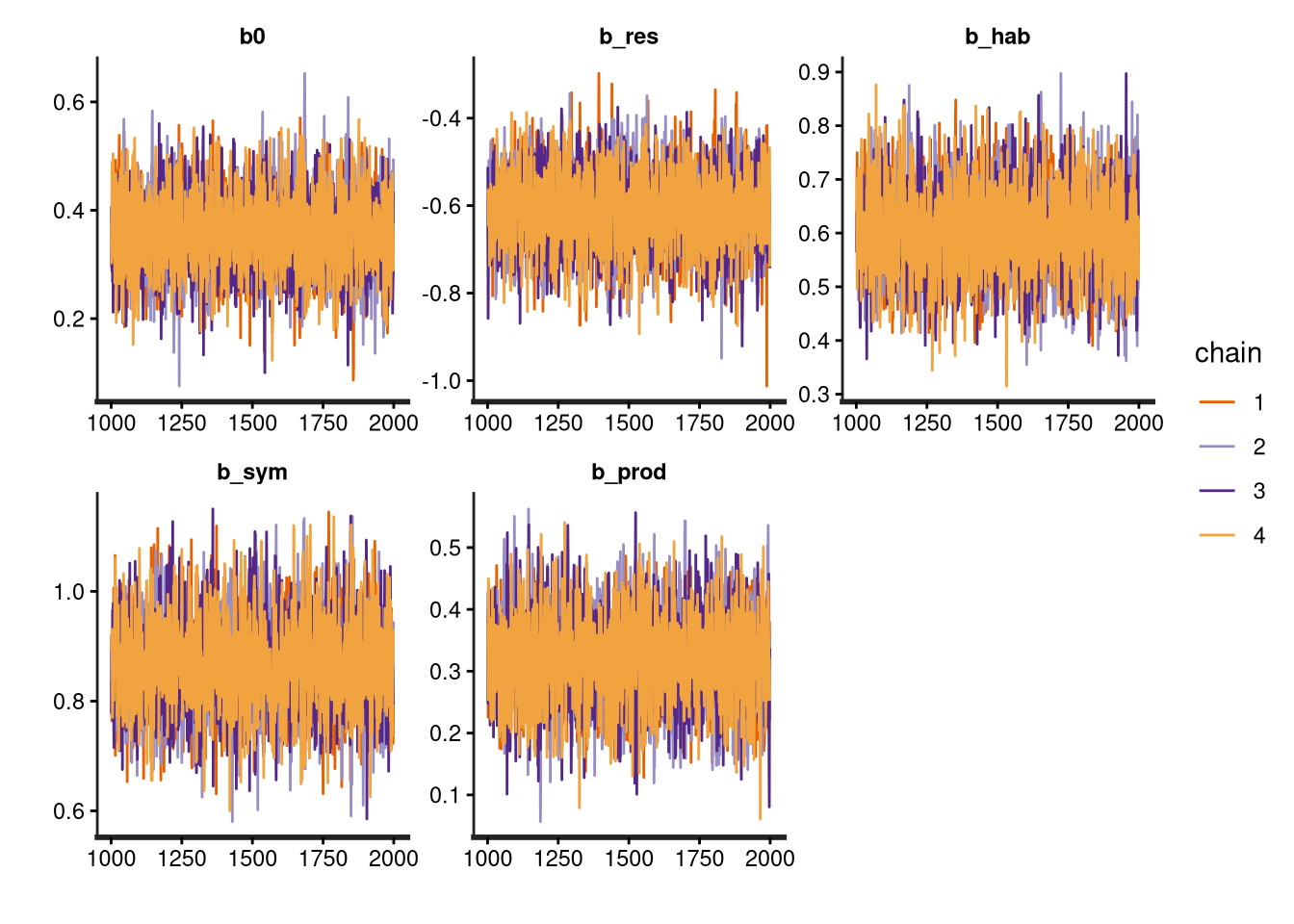

All chains have converged nicely!

print(precis(out_routes, pars = c("b0", "b_res", "b_hab", "b_sym", "b_prod")))

             mean         sd       5.5%      94.5%    n_eff     Rhat4
b0      0.3580424 0.07348836  0.2426148  0.4763884 4384.413 0.9993187
b_res  -0.6122113 0.08883884 -0.7535753 -0.4705709 4859.209 0.9993722
b_hab   0.6029176 0.08304119  0.4679325  0.7365925 4911.565 0.9994012
b_sym   0.8675144 0.08590655  0.7310412  1.0059165 4756.862 1.0005226
b_prod  0.3198335 0.07214356  0.2039426  0.4355752 4887.856 0.9991473

Our model estimates of the true parameters are mostly very good, however the intercept mean (baseline log-odds ratio) is slightly underestimated and the credible interval does not include the true value (0.5).

# Your true values in the exact order: b0, b_res, b_hab, b_sym, b_prod
true_values <- c(0.5, -0.7, 0.6, 0.8, 0.3)

# Corresponding base R y-coordinates (from top 5 down to bottom 1)
y_coords <- c(5, 4, 3, 2, 1)

plot(precis(out_routes, pars = c("b0", "b_res", "b_hab", "b_sym", "b_prod")),
     xlim = c(-1, 1),
     main = "Posterior Estimates vs. True Parameters")

abline(v = 0, lty = 2, col = "gray50") 
points(x = true_values, y = y_coords, col = "deepskyblue3", pch = 18, cex = 2)
legend("topright", legend = "True Parameter", col = "deepskyblue3", pch = 18, bty = "n")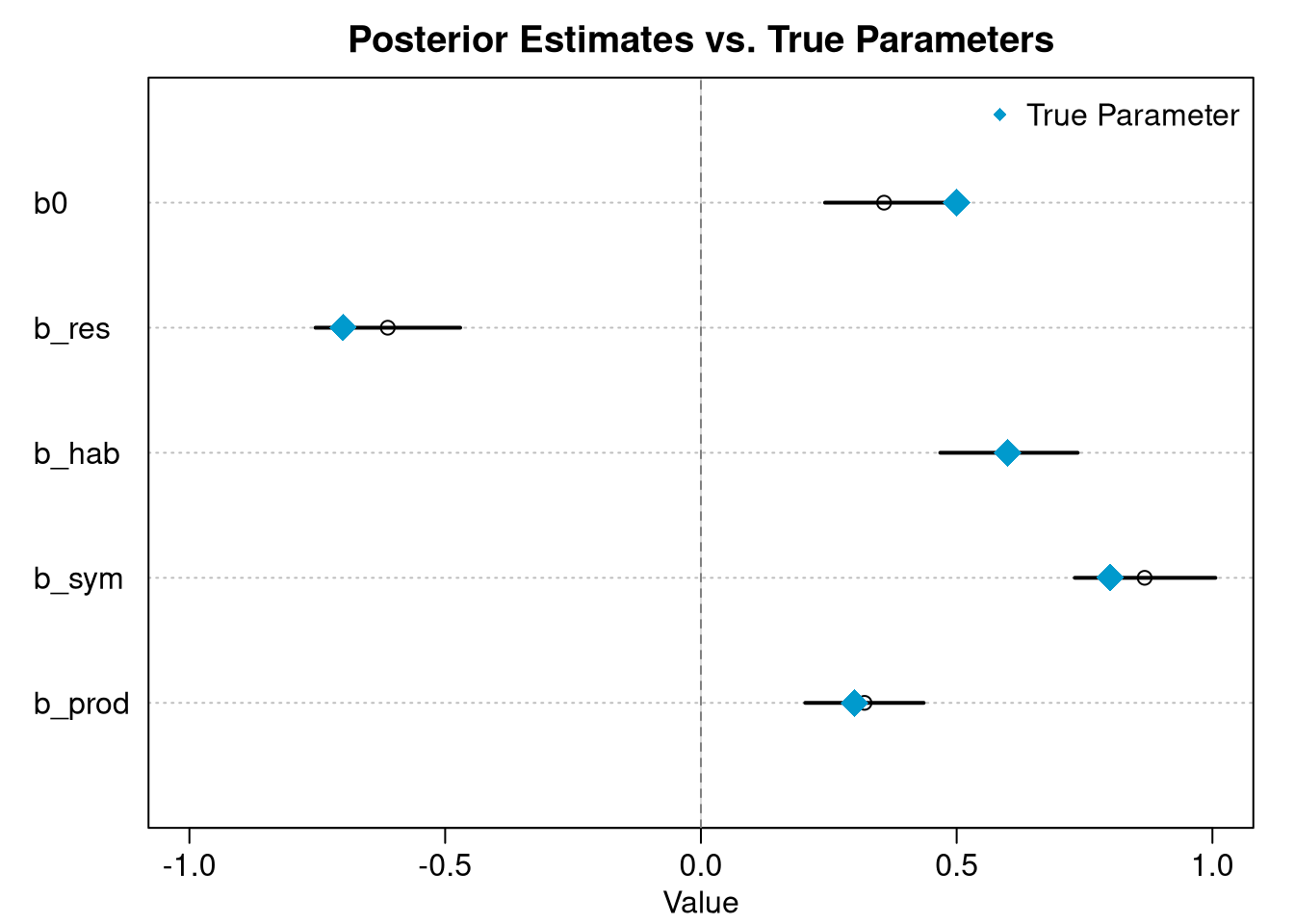

In this forest plot we can see, that all estimated values for the parameters lays in the credible interval, which means that there is an 89 % probability that the true effect sits inside this fixed window.

Why does rethinking uses 89% credible interval?

As Richard McElreath explains in Statistical Rethinking, the package uses 89% by default as a gentle scientific protest against the arbitrary nature of the traditional “95% p-value threshold.” 89 is also a prime number, which serves as a friendly reminder that credible intervals are continuous descriptions of uncertainty, not strict boundaries for what is “significant” and what isn’t!

3.2 Stop-Scale Model

I decided to use the hierarchical model accounting for stops association with the same route. Because nested sampling plots inherit shared local micro-habitats, spatial clustering, and unmeasured environmental noise, data points within the same route are non-independent. To account for this hierarchical structure without introducing sampling bottlenecks, the model employs an adaptive, non-centered group-level random effects architecture. This approach allows me to check if there is any significant variance among routes.

The Stop Scale model evaluates fine-scale species co-occurrence (syntopy) at localized survey points (\(i\)) nested within larger geographic scale (routes):

\[\text{log}(\alpha_i) = \beta_{0} + \beta_{res.div} \cdot X_{1,i} + \beta_{hab.pref} \cdot X_{2,i} + \beta_{prod} \cdot X_{3,i} + \beta_{sympatry} \cdot X_{4,i} + (z_{\text{route}[i]} \times \sigma_{\text{route}})\]

Presuming, that the variation among routes is highly clustered close to zero, we need to specify two adaptive priors to eliminate the geometric restrictions of “Neal’s Funnel” near zero variance during Hamiltonian Monte Carlo sampling (see box 4). The group-level deviations are mathematically decoupled into a standardized multiplier vector (\(z_{\text{route}}\)) and a global variance scaling parameter (\(\sigma_{\text{route}}\)):

\[z_{\text{route}[i]} \sim \text{Normal}(0, 1)\]

\[\sigma_{\text{route}} \sim \text{Exponential}(1)\]

# Map character route IDs to sequential integers for Stan indexing
stop_data$route_index <- as.integer(as.factor(stop_data$route_id))

dat_list_stops <- list(
  k_stops     = stop_data$k_stops,
  m1_stops    = stop_data$m1_stops,
  m2_stops    = stop_data$m2_stops,
  S_total     = stop_data$S_total,
  res_div     = stop_data$res_div,
  hab_pref    = stop_data$hab_pref,
  prod        = stop_data$prod,
  sympatry    = stop_data$sympatry,
  route_index = stop_data$route_index
)

# Model Settings
model_stops <- ulam(
  alist(
    # Likelihood using stop-level data arrays
    k_stops ~ custom( fisher_hyper_lpmf(k_stops[i] | exp(log_omega[i]), m1_stops[i], m2_stops[i], S_total[i]) ),
    
    # Linear Predictor: Pair baseline + Route random effect deviation
log_omega <- b0 + b_res*res_div + b_hab*hab_pref + b_prod*prod + b_sym*sympatry + (z_route[route_index] * sigma_route),

    # Fixed Effect Priors
    b0 ~ dnorm(0, 3),
    b_res ~ dnorm(0, 3),
    b_hab ~ dnorm(0, 3),
    b_sym ~ dnorm(0, 3),
    b_prod ~ dnorm(0, 3),
    
    # Adaptive Priors
    # Non-Centered Random Effect Layer
    # z_route is a completely standard, clean vector array
    z_route[route_index] ~ dnorm(0, 1),
    sigma_route ~ dexp(1)
    # exponential distribution forces sigma_route
    # to be strictly positive (since a standard deviation cannot be negative)
  ), 
  data = dat_list_stops, 
  sample = FALSE # Generate text for stan, not sampling yet
)

# Extract the autogenerated text
stan_code_stops <- stancode(model_stops)

# Paste the file-loaded functions block to the top of the text string
full_stan_code_stops <- paste0(likelihood_pmf, "\n", stan_code_stops)

# Run the compiled model using rstan
out_stops <- stan(
  model_code = full_stan_code_stops,
  data = dat_list_stops,
  chains = 4, 
  cores = 4,
  iter = 2000,
  seed = 1
)

Box 4: Non-centered Parameterization

Hierarchical models with group-level random effects often suffer from severe geometric pathologies during Hamiltonian Monte Carlo sampling, a phenomenon known as Neal’s Funnel. This issue arises when data provide weak information about group-level variance (\(\sigma_{\text{route}}\)), forcing the sampler to explore regions where the parameter space drastically constricts near zero.

To evaluate whether our choice of model architecture was necessary, we can visually compare the geometry Stan had to explore before and after the non-centered transformation. We will use for this libraries ggplot2 and bayesplot.

# Extract posterior samples
posterior_samples <- as.data.frame(out_stops)

# Extract the original effect for selected route
posterior_samples$alpha_route_1 <- posterior_samples$`z_route[1]` * posterior_samples$sigma_route

# Visual check of Neal's Funnel
ggplot(posterior_samples, aes(x = alpha_route_1, y = sigma_route)) +
  geom_hex(bins = 50) + 
  scale_fill_viridis_c(option = "plasma") +
  labs(
    title = "Parameters Check for Neal's Funnel",
    x = "Route effect (alpha_route = z_route * sigma_route)",
    y = "Variability among routes (sigma_route)"
  ) +
  theme_minimal()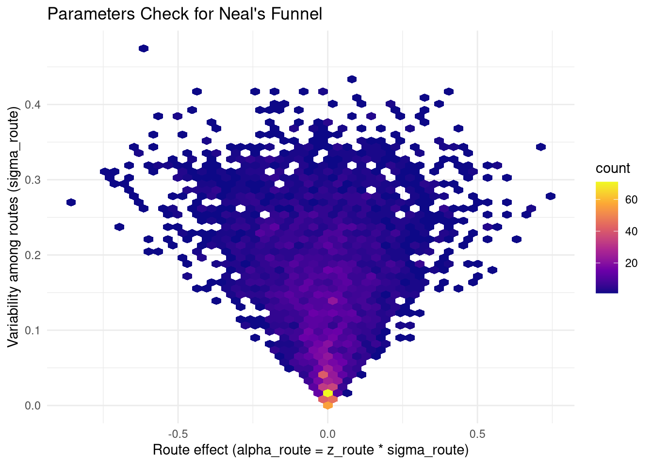

# Visual check of the effect of non-centered parametrization
ggplot(posterior_samples, aes(x = `z_route[1]`, y = sigma_route)) +
  geom_hex(bins = 50) + 
  scale_fill_viridis_c(option = "plasma") +
  labs(
    title = "Effect of Non-centered Parametrization (Stop-Scale Model)",
    x = "Standardised route effect (z_route[1])",
    y = "Variability among routes (sigma_route)"
  ) +
  theme_minimal()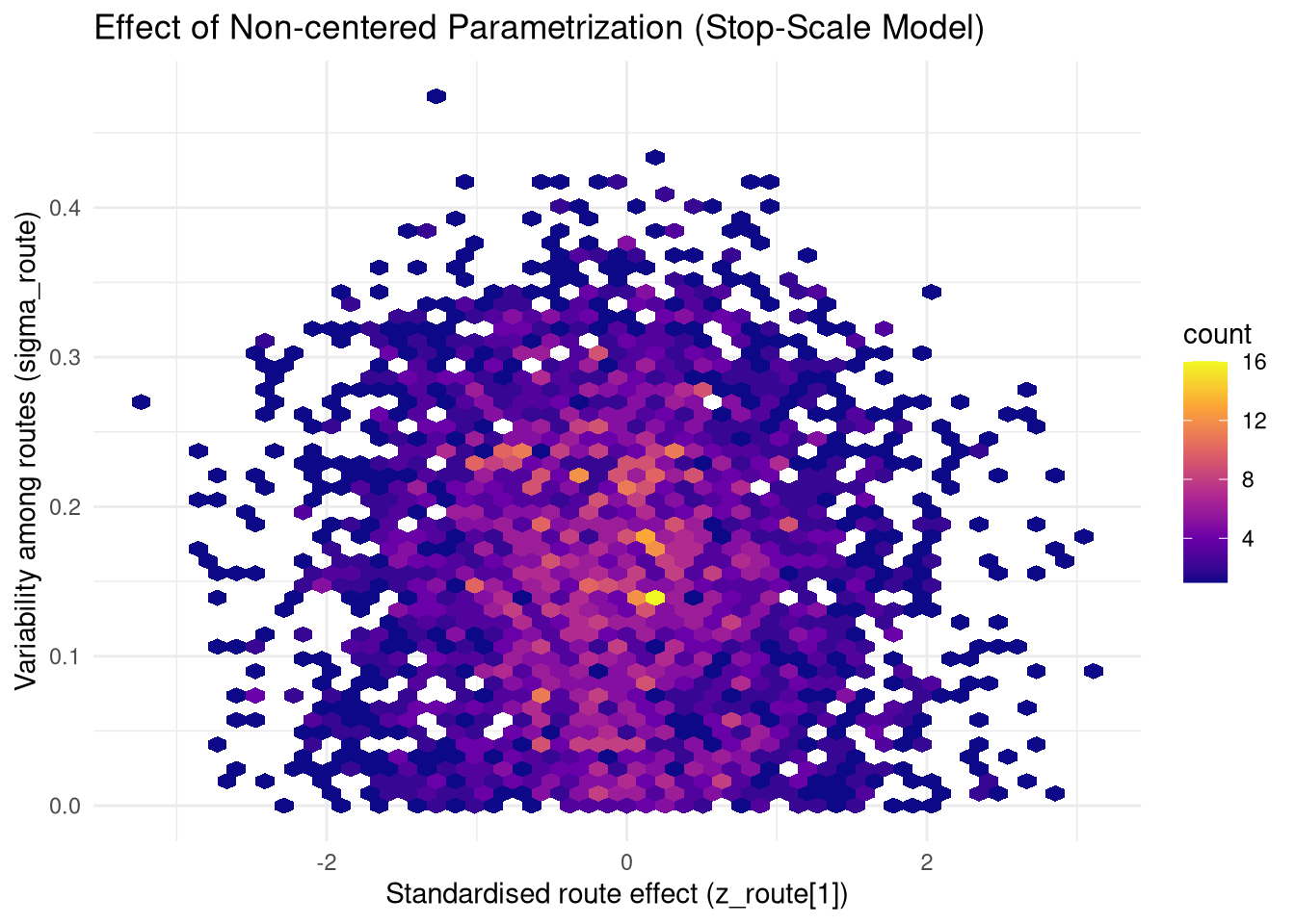

We can see, that the non-centered parameterization was definitely the right choice in this case.

First, we check the convergence with traceplot() for the main parameters.

traceplot(out_stops, pars = c("b0", "b_res", "b_hab", "b_sym", "b_prod", "sigma_route"))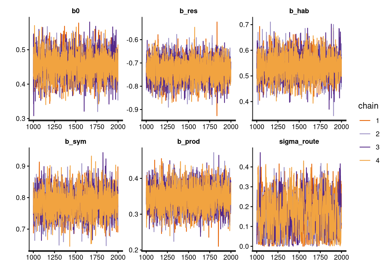

The convergence for sigma_route looks a bit suspicious. Let us check the main parameter estimates.

print(precis(out_stops, pars = c("b0", "b_res", "b_hab", "b_sym", "b_prod", "sigma_route")))

                  mean         sd        5.5%      94.5%     n_eff     Rhat4
b0           0.4545767 0.03729505  0.39508953  0.5134662 5927.4645 0.9996643
b_res       -0.7305365 0.04960014 -0.81025173 -0.6518122 6332.1603 0.9995585
b_hab        0.5378198 0.04716775  0.46384578  0.6125945 4737.9331 0.9992167
b_sym        0.7832212 0.03973275  0.71928783  0.8460992 7113.1752 0.9995082
b_prod       0.3457152 0.03525719  0.29053240  0.4023842 5497.5393 0.9998219
sigma_route  0.1642035 0.09395878  0.01898218  0.3180582  699.6114 1.0126586

The stop-scale model estimated the fixed effects with high precision, yielding well-mixed chains (\(\hat{R} < 1.00\) and high \(n_{eff}\) for all main predictors). The variance between routes is negligible, indicating that the adaptive prior successfully shrunk localized deviations back to the global environmental baseline (see box 5 for details).

Box 5: Local Route Effect

color_scheme_set("green")
mcmc_hist(out_stops, pars = c("b0", "b_res", "b_hab", "b_sym", "b_prod", "sigma_route"))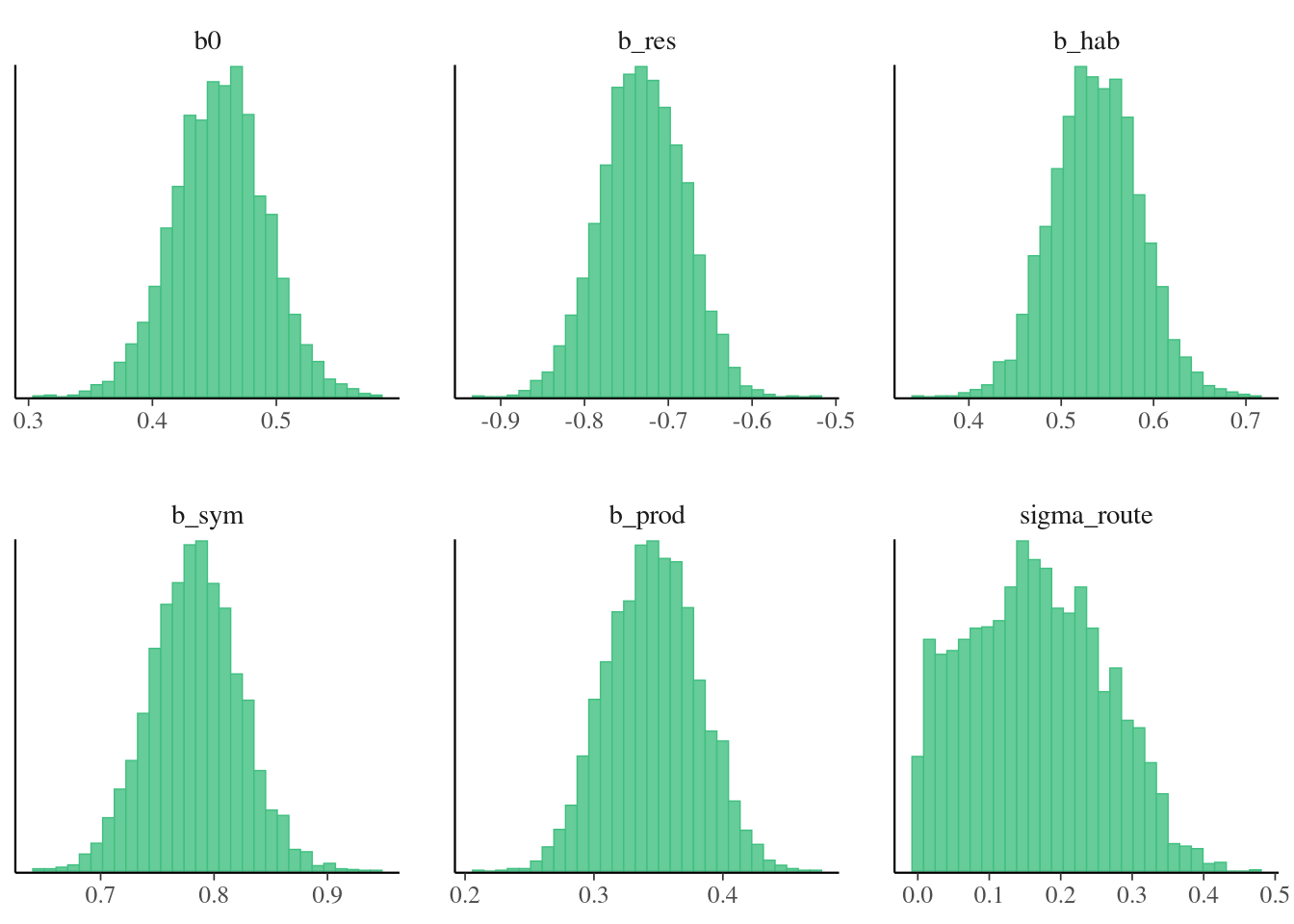

The estimated global standard deviation between routes (\(\sigma_{route}\)) had a posterior mean of \(0.16\) (\(89\%\) CI: \([0.02, 0.32]\)). This local route effect was created earlier using beta distribution (\(\theta = 5\)) for local point occupancy probabilities with the pair’s regional rates as \(\mu\).

Quantitatively, this indicates that the route-level random effect accounts for minor residual variation. A \(\sigma_{route}\) of \(0.16\) translates to a subtle \(\approx 17\%\) shift (\(e^{0.16}\)) in the co-occurrence odds ratio between typical routes. In contrast, fixed environmental and macro-ecological predictors—such as sympatry (\(b_{sym} = 0.78\), corresponding to a \(>118\%\) increase in odds) and habitat preference (\(b_{hab} = 0.54\)) — exerted a substantially stronger influence on fine-scale syntopy.

While the slightly lower effective sample size (\(n_{eff} \approx 700\)) and marginal \(\hat{R} = 1.01\) for \(\sigma_{route}\) suggest that the data are relatively uninformative about the exact scale of route-level variance, the posterior successfully concentrates near zero. This indicates that after controlling for key environmental covariates, macro-scale geographic grouping introduces negligible residual spatial clustering.

We now compare model estimations of syntopy (log-OR) with the true values we stated for the simulation of the data.

# Extract posterior sample draws
post_stops <- extract.samples(out_stops)
n_samples  <- length(post_stops$b0)
n_rows     <- nrow(stop_data)

# Create an empty matrix to hold log-odds (rows = post-samples, cols = stop_data rows)
log_alpha_routes <- matrix(NA, nrow = n_samples, ncol = n_rows)

# Reconstruct log_alpha per transect by pulling pair fixed effects and adding local random noise
for(i in 1:n_rows) {
  pair_base <- post_stops$b0 + 
               post_stops$b_res * stop_data$res_div[i] + 
               post_stops$b_hab * stop_data$hab_pref[i] + 
               post_stops$b_sym * stop_data$sympatry[i] + 
               post_stops$b_prod * stop_data$prod[i]
  
  # Manually reconstruct the route deviation from the non-centered samples
  current_route_idx <- stop_data$route_index[i]
  reconstructed_a_route <- post_stops$z_route[, current_route_idx] * post_stops$sigma_route
  
  # Total local log-odds ratio
  log_alpha_routes[, i] <- pair_base + reconstructed_a_route
}

# Compute and assign the estimated log-odds ratio back to each individual transect row
stop_data$estimated_local_log_OR <- colMeans(log_alpha_routes)

# Average the estimated log-odds values for each distinct pair_id
pair_level_averages <- aggregate(estimated_local_log_OR ~ pair_id, data = stop_data, FUN = mean)
stop_model_evaluation <- pair_level_averages |> 
  left_join(route_data |> select(pair_id, true_log_OR = log_OR), by = "pair_id")
head(stop_model_evaluation)

pair_id	estimated_local_log_OR	true_log_OR
1	0.3525804	0.4148120
2	0.4569615	0.3835914
3	-0.1700722	-0.0188833
4	0.3889530	0.3964178
5	1.8044773	1.8454474
6	-0.3685949	-0.2967890

Apparently, our model estimations of true log-odds ratio are mostly very precise. We can also plot it.

plot(stop_model_evaluation$true_log_OR, stop_model_evaluation$estimated_local_log_OR,
     pch = 16, col = rgb(0.1, 0.4, 0.7, 0.6), cex = 1.2,
     xlab = "True Log-Odds Ratio (Generated)",
     ylab = "Model-Estimated Log-Odds Ratio",
     main = "Posterior Predictive Validation (Stop Scale)")

# Add a 1:1 line of perfect recovery
abline(a = 0, b = 1, lty = 2, lwd = 2, col = "darkgray")

# Add a smooth trendline of actual estimates
abline(lm(estimated_local_log_OR ~ true_log_OR, data = stop_model_evaluation), 
       col = "firebrick", lwd = 2)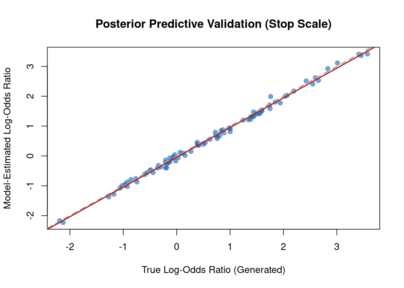

Finally, we can plot the comparison of our posterior from stop scale model with the true parameter values.

# Your true values in the exact order: b0, b_res, b_hab, b_sym, b_prod
true_values <- c(0.5, -0.7, 0.6, 0.8, 0.3)

# Corresponding base R y-coordinates (from top 5 down to bottom 1)
y_coords <- c(5, 4, 3, 2, 1)

plot(precis(out_stops, pars = c("b0", "b_res", "b_hab", "b_sym", "b_prod")),
     xlim = c(-1, 1),
     main = "Posterior Estimates vs. True Parameters")

abline(v = 0, lty = 2, col = "gray50") 
points(x = true_values, y = y_coords, col = "deepskyblue3", pch = 18, cex = 2)
legend("topright", legend = "True Parameter", col = "deepskyblue3", pch = 18, bty = "n")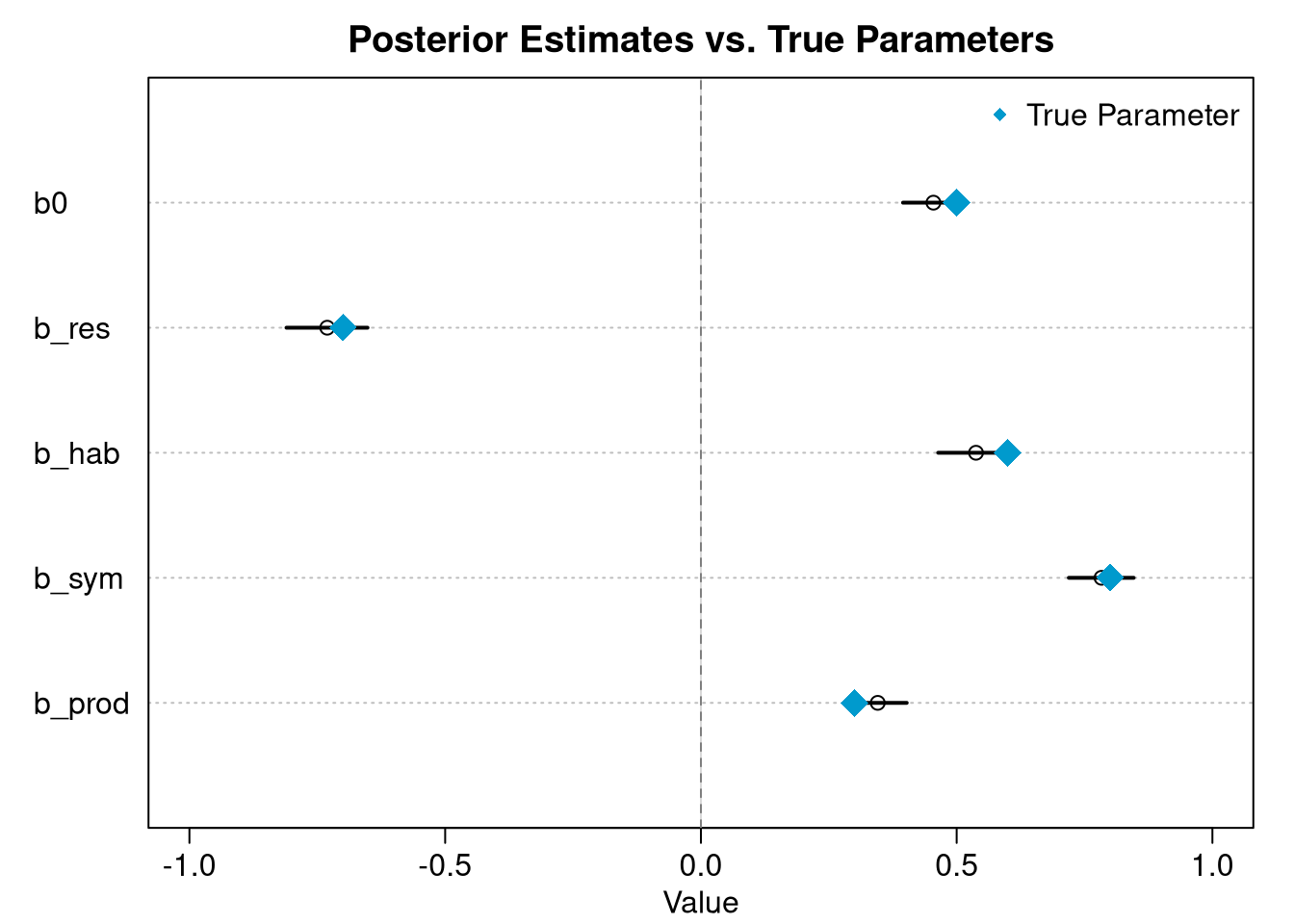

Supplementary Analysis: 30-Pair Downscaled Simulation

To evaluate how model performance scales with a smaller dataset, I wrapped our exact data-generating process into a function and simulated data for only 30 species pairs.

source("simulate_stop_data.R")
dat_list_stops_sample <- simulate_stop_data(num_pairs = 30)

model_stops_sample <- ulam(
  alist(
    k_stops ~ custom( fisher_hyper_lpmf(k_stops[i] | exp(log_omega[i]), m1_stops[i], m2_stops[i], S_total[i]) ),
    log_omega <- b0 + b_res*res_div + b_hab*hab_pref + b_prod*prod + b_sym*sympatry + (z_route[route_index] * sigma_route),
    b0 ~ dnorm(0, 3),
    b_res ~ dnorm(0, 3),
    b_hab ~ dnorm(0, 3),
    b_sym ~ dnorm(0, 3),
    b_prod ~ dnorm(0, 3),
    z_route[route_index] ~ dnorm(0, 1),
    sigma_route ~ dexp(1)
  ), 
  data = dat_list_stops_sample, 
  sample = FALSE
)

full_stan_code_sample <- paste0(likelihood_pmf, "\n", stancode(model_stops_sample))
out_stops_sample <- stan(
  model_code = full_stan_code_sample,
  data = dat_list_stops_sample,
  chains = 4, cores = 4, iter = 2000, seed = 1
)

print(precis(out_stops_sample, pars = c("b0", "b_res", "b_hab", "b_sym", "b_prod", "sigma_route")))

                  mean         sd         5.5%      94.5%     n_eff     Rhat4
b0           0.4969248 0.06471253  0.393554818  0.5984242 3233.9959 0.9999493
b_res       -0.6404466 0.06928092 -0.751189187 -0.5285713 4422.4810 1.0007039
b_hab        0.5684211 0.07067034  0.455209411  0.6837015 4326.8120 0.9999351
b_sym        0.8490875 0.05791267  0.759287490  0.9419850 2970.9032 1.0002581
b_prod       0.2966673 0.05239861  0.213702279  0.3825593 3367.7119 1.0001228
sigma_route  0.1022434 0.07663798  0.009139228  0.2450797  888.9829 1.0033985

We can see that the model is more certain and \(\mu\) for \(\beta_{sympatry}\) is estimated precisely.

true_values <- c(0.5, -0.7, 0.6, 0.8, 0.3)

# Corresponding base R y-coordinates (from top 5 down to bottom 1)
y_coords <- c(5, 4, 3, 2, 1)

plot(precis(out_stops_sample, pars = c("b0", "b_res", "b_hab", "b_sym", "b_prod")),
     xlim = c(-1, 1),
     main = "Posterior Estimates vs. True Parameters")

abline(v = 0, lty = 2, col = "gray50") 
points(x = true_values, y = y_coords, col = "deepskyblue3", pch = 18, cex = 2)
legend("topright", legend = "True Parameter", col = "deepskyblue3", pch = 18, bty = "n")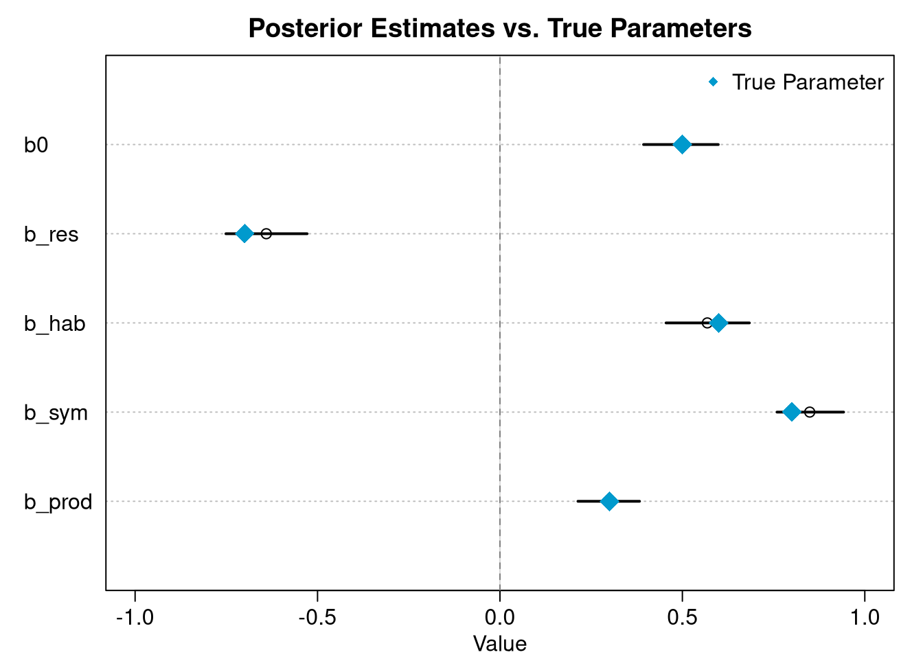

Coding Workflow

I used Gemini 3.5 to enhance plots and help with some of the stuff in this assignment, like writing the likelihood function or function for stop scale data generation. I always reviewed the AI output and tried to apply the approaches learned in the course as much as possible.

4 Conclusion

This assignment was about simulating syntopy dataset using generative parameters tuned to reflect established ecological thresholds and known structure design of BBS data. I simulated data for route and stop scale, assuming there is no difference in the true values of parameters between scales. Than I tried to estimate back the specifed true values using Bayesian model for each scale separately.

Both models estimated the true values for \(\text{N} = 100\) with sufficient precision, although the route-scale model slightly underestimated the baseline syntopy (true \(\beta_{0}=0.5\); route-scale model: \(\mu = 0.36\), \(\sigma = 0.07\) (\(89\%\) CI: \([0.24, 0.48]\)). The stop-scale model estimated syntopy much more accurately (\(\mu = 0.45\), \(\sigma = 0.04\) (\(89\%\) CI: \([0.40, 0.51]\)) and showed that the variance among routes is very small, suggesting minor sampling noise. I also checked the effect of a smaller sample size (\(\text{N} = 30\)) on the parameter estimates, for which \(\beta_{sympatry}\) was also estimated with a sufficient precision (\(\mu = 0.49\), \(\sigma = 0.06\) (\(89\%\) CI: \([0.39, 0.59]\)).

5 References

McGeoch, Melodie A., and Kevin J. Gaston. 2002. “Occupancy Frequency Distributions: Patterns, Artefacts and Mechanisms.” Biological Reviews 77 (3): 311–31. https://doi.org/10.1017/S1464793101005887.

Newbury, Arthur. 2025. “Bayesian Estimation of Co-Occurrence Affinity with Dyadic Regression.” bioRxiv, ahead of print. https://doi.org/10.1101/2024.01.16.575941.

Remeš, Vladimír, and Lenka Harmáčková. 2023. “Resource Use Divergence Facilitates the Evolution of Secondary Syntopy in a Continental Radiation of Songbirds (Meliphagoidea): Insights from Unbiased Co-Occurrence Analyses.” Ecography 2023 (2): e06268. https://doi.org/10.1111/ecog.06268.

Remeš, Vladimír, and Lenka Harmáčková. 2025. “Completing the Speciation Cycle: Ecological Niches and Traits Predict Local Species Coexistence in Birds Across the Globe.” Global Ecology and Biogeography 34 (2): e70002. https://doi.org/10.1111/geb.70002.